The IS-LM Model as a Tool for Effective Policymaking : Fiscal and Monetary Policy

The analysis of fiscal and monetray policy is important for macroeconomic stability especially price stability and sustailed economic growth. Fiscal and monetary policies differ with each other in the sense that generally fiscal policy refers to to the government’s distribution and taxation policy to achieve economic growth, on the other hand, the basic component of monetary policy is to control inflation or more precisely price stability and controlling money supply in the economy.

As we know from keynesian macroeconomic analysis there is diffrent market for goods and money that is, 1) Goods Market 2) Money market.
And according to Keynes, when aggregate demand that is sum of consumption dermand, investment demand, government expenditure and net exports equals the national income or GDP. When this aggregate demand equals the aggregate supply goods market is in equilibrium.

On the other hand, money market is in eqilibrium when demand for money that is liquidity preference is equals to the supply of money.

The importantce of IS-LM curve is that it synthesises the goods market and money market and simultanously determine its equlibrium through its interaction of IS and LM curve. And importantce of this approach is that it helps the policymakers to formulate policies of fiscal and monetary according to IS-LM curve analysis.

This article delves into the world of the IS-LM model, exploring its key components and their interaction. We’ll see how the model depicts the interplay between investment, saving, interest rates, and the money supply. Through this lens, we’ll examine how policymakers can leverage fiscal tools like government spending and taxes, as well as monetary instruments like interest rate adjustments and money supply manipulation, to achieve their desired economic outcomes.

The IS-LM model, while a simplified representation, offers valuable insights. It allows us to visualize the impact of policy changes on key economic variables, such as output and interest rates. This understanding empowers policymakers to make informed decisions, fostering economic stability and promoting long-term growth.

As we delve deeper, we’ll not only explore the effectiveness of each policy type but also uncover the potential limitations of the IS-LM model. Recognizing these limitations allows for a more nuanced understanding of the real-world economy, where factors beyond the model’s scope can influence outcomes.

By the end of this explanation, we gain a deeper appreciation for the IS-LM model and its significance in the realm of effective policymaking.

What is IS-LM Curve?

In the “General Theory of Interest and Money” Keynes explained the goods market and money market equilibrium seperately. And criticised the classical economists of self correcting economic model and full employment of resources. According to the Keynes, the private enterprise economy is not self correcting as well as there is no gurantee about always full employment in the economy. However with active fiscl and monetary policies economy can be in equlibrium position.

While Keynes determined goods market equilibrium in the way that aggregate demand is equals aggregate supply where aggregate demand is the sum of consumption demand, investment demand, government expanditure a nd net exports. It is important to note that investment demand is the autonomus or independend demand that is it is taken as the independent variable. On the other hand, money market equlibrium is established when demand for money that is liquidity preference equals supply for money. As far as Keynes analysis considered, according to Keynes, in the short run supply of money is fixed hence demand for money fluctuates in the short period. Now the demand for money or what keynes called liquidity preference depends upon three motives — 1) Transaction Motive 2)Precautionary Motive 3) Speculative motive.
However, there is a basic flow in the Keynesian goods market and money market equilibrium analysis. Keynes disregarded the effects of money market equilibrium to that of goods market hence some modern economists — J.R.Hicks, Hansen tries to extend this Keynesian analysis of goods market and money market with integrating both markets.

Understanding the IS-LM Model: A Breakdown

The IS-LM model, also known as the Hicks-Hansen model, is a fundamental tool in Keynesian economics. It’s a two-dimensional framework that depicts the interaction between the real sector of the economy (goods and services market) and the monetary sector (money market) in the short run. By analyzing the intersection of two key curves, the IS curve and the LM curve, we can understand how interest rates and real GDP are determined.

1. The IS Curve (Investment-Savings)

The IS curve represents all combinations of real GDP (Y) and interest rates (i) where planned investment equals planned saving. In simpler terms, it shows the level of economic output at which businesses’ desired investment matches what households are willing to save.

Relationship to Interest Rates: As interest rates rise, borrowing becomes more expensive, and businesses tend to invest less. This relationship creates a downward slope for the IS curve. Higher interest rates correspond to lower real GDP levels on the curve.
Relationship to Real GDP: When real GDP rises, businesses generally become more optimistic and increase investment. This upward shift in investment spending pushes the IS curve to the right, indicating higher real GDP at each interest rate level.

2. The LM Curve (Liquidity Preference-Money Supply)

The LM curve represents all combinations of real GDP (Y) and interest rates (i) where the demand for money equals the supply of money. It essentially shows the relationship between interest rates and how much money people want to hold.

Relationship to Interest Rates: As interest rates rise, holding money becomes more attractive compared to investing in bonds or other interest-bearing assets. This increased demand for money pushes the LM curve upwards. Higher interest rates correspond to higher money demand on the curve.
Relationship to Money Supply: An increase in the money supply by the central bank allows people to hold more money at any given interest rate. This shift in supply pushes the LM curve to the right, indicating more money being demanded at each interest rate level.

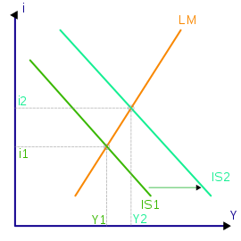
3. Interaction and Equilibrium

The IS and LM curves come together to determine the equilibrium levels of real GDP (Y*) and interest rate (i*). Here’s how:

Intersection Point: The intersection point of the IS and LM curves represents the simultaneous equilibrium in both the goods and money markets. At this point, both planned investment equals planned saving (IS curve) and the demand for money equals the supply of money (LM curve).
Impact of Shifts: Changes in fiscal policy (government spending or taxes) or monetary policy (money supply or interest rates) can cause the IS or LM curves to shift, leading to new equilibrium levels of real GDP and interest rates. For instance, an increase in government spending would shift the IS curve to the right, indicating higher real GDP and potentially higher interest rates at the new equilibrium.

In essence, the IS-LM model provides a simplified framework to analyze the impact of various factors on economic activity (real GDP) and the cost of borrowing (interest rates). Remember, the model focuses on the short-run where prices are sticky, and it has limitations in representing complex economic scenarios.

Analyzing Fiscal Policy with the IS-LM Model — Fiscal policy refers to the use of government spending and taxes to influence economic activity. The IS-LM model helps us understand how these policies can impact real GDP and interest rates.

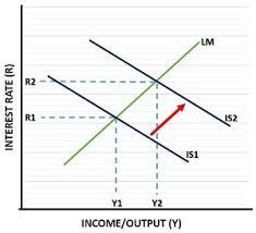
Impact on IS Curve

Government Spending: An increase in government spending injects additional money into the economy, directly boosting aggregate demand. This upward shift in investment due to higher government expenditure pushes the IS curve to the right. Conversely, a decrease in government spending shifts the IS curve to the left.
Taxes: A decrease in taxes leaves more money in the hands of households and businesses, leading to higher investment and consumption. This upward movement in aggregate demand shifts the IS curve to the right. On the other hand, an increase in taxes reduces disposable income, causing a downward shift in the IS curve to the left.

Fiscal Multipliers —

Fiscal policy can have a magnified effect on real GDP beyond the initial change in government spending or taxes. This amplification is captured by the concept of fiscal multipliers.

Fiscal Multiplier: When the government injects money into the economy through spending or tax cuts, it creates a ripple effect. People and businesses receiving the additional income are likely to spend a portion of it, which in turn leads to increased spending by others in the economy. This chain reaction ultimately leads to a larger increase in real GDP compared to the initial fiscal stimulus.
Factors Affecting Multipliers: The size of the fiscal multiplier depends on several factors, including the marginal propensity to consume (MPC). MPC refers to the proportion of additional income that people choose to spend. A higher MPC leads to a larger multiplier effect, as more spending rounds occur in the economy.

The IS-LM model provides a framework to analyze how fiscal policy influences real GDP and interest rates. By understanding the shifts in the IS curve caused by government spending and taxes, we can predict the overall impact on economic activity. Fiscal multipliers add another layer of complexity, highlighting the potential for amplified effects of fiscal policy through the spending chain reaction.

Analyzing Monetary Policy with the IS-LM Model — Monetary policy refers to the actions taken by the central bank to influence economic activity and inflation. The IS-LM model helps us understand how the central bank’s tools, particularly open market operations, affect real GDP and interest rates.

Open Market Operations and the LM Curve

Open market operations (OMO) are the central bank’s primary tool for influencing the money supply. Here’s how they impact the LM curve:

Open Market Purchase: When the central bank purchases government bonds from the public, it injects new money into the economy by increasing bank reserves. This increase in money supply pushes the LM curve to the right, indicating more money available at each interest rate level.
Open Market Sale: Conversely, selling government bonds to the public reduces bank reserves and the money supply. This shift in supply pushes the LM curve to the left, indicating less money available at each interest rate level.

Money Supply, Interest Rates, and Real GDP

Changes in the money supply caused by OMOs affect interest rates and real GDP through the IS-LM framework:

Lower Interest Rates: An increase in money supply pushes the LM curve to the right, lowering interest rates at the intersection point with the IS curve. Lower interest rates encourage borrowing and investment, leading to higher real GDP (expansionary effect).
Higher Interest Rates: A decrease in money supply (leftward shift of LM curve) increases interest rates, discouraging investment and potentially reducing real GDP (contractionary effect).

The impact on real GDP can be amplified by the presence of liquidity preference. When interest rates fall, people might prefer to hold more money instead of spending it, dampening the initial boost to real GDP.

Interest Rate Adjustments —

While OMOs are the primary tool for managing the money supply, central banks can also directly influence interest rates through the:

Discount Rate: This is the rate at which commercial banks borrow reserves from the central bank. Adjusting the discount rate can incentivize or discourage banks from borrowing reserves, impacting the overall money supply and interest rates in the economy.
Reserve Requirements: This is the minimum amount of reserves that banks must hold against deposits. Changing reserve requirements directly affects the money supply available for lending, influencing interest rates.

However, in the IS-LM framework, these tools often achieve similar results as OMOs by indirectly influencing the money supply and ultimately impacting the LM curve.

Limitations of the IS-LM Model: A Look Beyond the Simplistic Framework- The IS-LM model is a powerful tool for understanding the interaction between the real and monetary sectors of the economy. However, it’s important to recognize that it’s a simplified framework with limitations that may not fully capture the complexities of the real world.

Here are some key limitations to consider:

Short-Run Focus: The IS-LM model primarily focuses on the short-run, where prices are assumed to be sticky. In the long run, prices adjust, and the model’s predictions become less accurate.
Perfect Capital Mobility: The model assumes perfect capital mobility, meaning money can freely flow across borders. This assumption doesn’t always hold true in the real world, where capital controls and exchange rate fluctuations can affect the effectiveness of monetary policy.
Neglect of Expectations: The model doesn’t explicitly consider how expectations of future economic conditions can influence behavior in the present. For instance, businesses and households might adjust their investment and spending decisions based on their expectations of future interest rates or inflation.
Limited Role of Government: The model treats government spending and taxes as exogenous variables, not considering how government policy itself might respond to changes in the economy.

By understanding the limitations of the IS-LM model and exploring alternative models, economists can gain a more complete picture of how the economy functions and make more informed policy decisions.

Conclusion — The IS-LM model provides a valuable framework for understanding the interaction between the real and monetary sectors of the economy. By analyzing the interplay of the IS curve (representing goods market equilibrium) and the LM curve (representing money market equilibrium), we can gain insights into how interest rates and real GDP are determined. This knowledge is crucial for policymakers aiming to influence economic activity and achieve desired outcomes.

While the model offers a simplified view, it highlights the importance of both fiscal and monetary policy in managing the economy. Fiscal policy, through government spending and taxes, can be used to stimulate growth or control inflation, but it’s subject to political considerations and time lags. Monetary policy, primarily through adjustments in interest rates and money supply, offers a quicker response but can have limitations, impacting growth and potentially triggering unintended consequences.

The effectiveness of each policy type depends on the specific economic situation and goals. Ideally, policymakers should use a combination of fiscal and monetary tools, considering their strengths and weaknesses. Recognizing the limitations of the IS-LM model, such as its short-run focus and neglect of expectations, is also crucial. Exploring alternative models that incorporate these complexities can provide a more complete picture for informed policy decisions.

The ongoing debate among economists regarding the optimal mix of fiscal and monetary policy underscores the need for continuous analysis and adaptation. As economic landscapes evolve, policymakers must remain flexible and employ a combination of tools to navigate challenges and promote a stable and prosperous economy. By understanding the IS-LM model as a stepping stone and acknowledging its limitations, we can strive for more effective policymaking that fosters long-term economic well-being.

Thanks.

Pratik Ghansham Salvi Assistant Professor of Economics | Banking & Finance | IMF Finance & Development Contributor

The IS-LM Model as a Tool for Effective Policymaking : Fiscal and Monetary Policy